PydanticAI + MCP + Ollama examples for your local tool-use LLM

This blog post is for you if you’ve heard of the model context protocol (MCP) and are curious how you could implement something in Python such that you can try it with your local models that are capable of tool use, e.g. via Ollama. Maybe you even looked at the documentation but felt there still was something missing for you to get started?

At least that’s how I felt. The “easiest” / Stdio server verison worked immediately but when I wanted to use a HTTP server I was sort of stranded. It was unclear to me how to actually run the server and what the client needs where so it can successfully talk to the server. Don’t get me wrong, the MCP and PydanticAI documentation is pretty good, but things could always be easier, could they not? 😛 Maybe I’ll save you some time with this post.

Model Context Protocol?

The MCP is designed to create servers that provide resources, prompts and tools and client that know how to handle those. The tools are intended to be directly used by language models from the side of the client.

So the examples here will only make use of the tools part of the MCP.

Types of servers

There are two types: Stdio and HTTP MCP servers. In my repo is one example for the Stdio type and three for the HTTP type, using mcp.run directly, or FastAPI or Starlette. You can find those in the following repo folders

Differences in Code

Following are the main differences in the implementation as I see them. For a more complete picture I recommend the links above and file diffs. 🙂

Client side

# stdio / subprocess server
def get_stdio_mcp_server() -> MCPServerStdio:
    return MCPServerStdio("uv", args=["run", "server.py", "server"])

# http server: mcp.run / fastapi / starlette
def get_http_mcp_server(port: int = PORT) -> MCPServerHTTP:
    return MCPServerHTTP(url=f"http://localhost:{port}/mcp")

For the Stdio server the client we need to define how to run the server.py script, e.g. using uv in def get_stdio_mcp_server above.

For the HTTP server we only need to provide the URL, but that URL needs to be correct. 😀 The last part of the path is important, otherwise you get irritating error messages.

Server side

The first example pretty much looks like

# examples/0_subprocess/server.py

from mcp.server.fastmcp import FastMCP
from typing import Literal

mcp = FastMCP("Stdio MCP Server") # server object

@mcp.tool() # register tool #1 
async def get_best_city() -> str:
    """Source for the best city"""
    return "Berlin, Germany"

Musicals = Literal["book of mormon", "cabaret"]

@mcp.tool() # register tool #2
async def get_musical_greeting(musical: Musicals) -> str:
    """Source for a musical greeting"""
    match musical:
        case "book of mormon":
            return "Hello! My name is Elder Price And I would like to share with you The most amazing book."
        case "cabaret":
            return "Willkommen, bienvenue, welcome! Fremde, étranger, stranger. Glücklich zu sehen, je suis enchanté, Happy to see you, bleibe reste, stay."
        case _:
            raise ValueError

mcp.run() # start the server

Quite beautifully easy.

The 1_http_mcp_run example is actually only a little bit different

# examples/1_http_mcp_run/server.py

# stuff

mcp = FastMCP(
    "MCP Run Server",
    port=PORT, # <- set this
)

# stuff

mcp.run(transport="streamable-http") # <- set this transport value

So mainly we have to set a port value and the transport value. Easy peasy.

What about fastapi / starlette + uvicorn?

# examples/2_http_fastapi/server.py - starlette version is very similar

# stuff

mcp = FastMCP(
    "MCP Run Server"
) # no port argument needed here

# stuff

@contextlib.asynccontextmanager
async def lifespan(app: FastAPI):
    async with contextlib.AsyncExitStack() as stack:
        await stack.enter_async_context(mcp.session_manager.run())
        yield

app = FastAPI(lifespan=lifespan) # try removing this and running the server ^^
app.mount("/", mcp.streamable_http_app())

uvicorn.run(app, port=PORT)

Well dang! Still relatively easy but some added work needed in defining the lifespan function and making sure the path is mounted correctly.

Running it

It’s documented here, but I’ve written the scripts such that all you need is python server.py and python client.py.

Then in your python client.py terminal it should look something like

If you use logfire as set up in the client.py scripts and register an account with logfire you should be able to see the prompts and responses neatly like

and

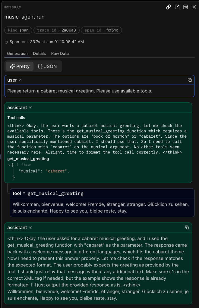
Auf Wiedersehen, au revoir, goodbye

That’s it. Happy coding! 🙂

Links to things

“hypermedia systems”‘s Contact.app with fasthtml

TL;DR

fasthtml is new, still seems to have some quirks, but is a great tool to use if you want to keep all your frontend logic in python.

Hello again

In my previous blog post I wrote about htmx used with flask and jinja2 as done by the authors of the book “hypermedia systems”.

Having done that one could wonder what that code would look like using fasthtml. This is what this blog post is about :), I know, you are probably shocked beyond belief, if you’ve seen my two previous posts.

Links to things

What is fasthtml?

According to the authors of fasthtml

with FastHTML you can get started on anything from simple dashboards to scalable web applications in minutes.

Bold claims. But the example they give in their docs illustrates the idea pretty well

from fasthtml.common import *
app = FastHTML()

@app.get("/")
def home():
    page = Html(
        Head(Title('Some page')),
        Body(Div('Some text, ', A('A link', href='https://example.com'), Img(src="https://placehold.co/200"), cls='myclass')))
    return page

serve()

So there is some similar routing as with flask, e.g. here with @app.get("/"). But then the great part that allows you to write frontend pieces is in the content of the function. That content is all you need to construct an actual HTML page, from python.

So all you need to learn is how fasthtml works to replace the jinja2 templating and html file business. The examples in their docs and their examples repo also are good starting points.

fasthtml to replace jinja2 templating and flask in the Contact.app

Was I successful swapping out jinja2 and flask with fasthtml? See for yourself :).

My attempt for this can be found in apps/web-fasthtml. It is based on apps/web4 ( so no json data api, but probably something that could be interesting to be done, especially with fastapi :P).

Turns out replacing the html / templating bits with fasthtml is relatively straigtforward, with a few quirks but also some pleasentness.

A good example of what the transition from jinja2 to fasthtml looks like is probably the HTML for the rows of the contacts to be displayed. In the original authors’ HTML that looks like

{% for contact in contacts %}
    <tr>
        <td><input type="checkbox" name="selected_contact_ids"
            value="{{ contact.id }}"></td>
        <td>{{ contact.first }}</td>
        <td>{{ contact.last }}</td>
        <td>{{ contact.phone }}</td>
        <td>{{ contact.email }}</td>
        <td>
            <a href="/contacts/{{ contact.id }}">View</a>
        </td>
        <td>
            <a href="/contacts/{{ contact.id }}/edit">Edit</a>
        </td>
        <td>
            <a
                href="#"
                hx-delete="/contacts/{{ contact.id }}"
                hx-swap="outerHTML swap:1s"
                hx-confirm="Are you sure you want to delete this contact?"
                hx-target="closest tr">Delete</a>
        </td>
    </tr>
{% endfor %}

with fasthtml it looks like

def get_rows(contacts: list[Contact]) -> FT:
    _get_td_view = lambda c: Td(A("View", href=f"/contacts/{c.id}"))
    _get_td_edit = lambda c: Td(A("Edit", href=f"/contacts/{c.id}/edit"))
    _get_td_delete = lambda c: Td(
        A(
            "Delete",
            href="#",
            hx_delete=f"/contacts/{c.id}",
            hx_swap="outerHTML swap:1s",
            hx_confirm="Are you sure you want to delete this contact?",
            hx_target="closest tr",
        )
    )
    rows = Tbody(
        Tr(
            Td(c.first),
            Td(c.last),
            Td(c.phone),
            Td(c.email),
            _get_td_view(c),
            _get_td_edit(c),
            _get_td_delete(c),
        )
        for c in contacts
    )
    return rows

So the order is a bit different, but pretty much 1:1 logic, except no knowledge of how jinja2 templating works is necessary, if you can figure out the proper way of passing arguments with fasthtml :D.

Quirks working with fasthtml

I see a few quirks when working with fasthtml, which may be worth knowing before diving in. Hopefully having read this it will save you some time down the line when you wonder why random 404s appear or data is not passed as expected.

Quirk #1 – Routing

In “hypermedia systems” a DELETE request to /contacts/archive triggers a dedicated function only for that combination of method and path. But in fasthtml this exact same code led to a 404 status code.

I may have overlooked fasthtml docs on how to properly fix this but I resorted to a dedicated path /contacts/archive/delete. That one actually was originally part of the vanilla HTML app but then actively removed in the “hypermedia systems” code in the book as a htmx feature.

This is what the htmx supported HTML looks like

<button hx-delete="/contacts/archive">
    Clear Download
</button>

This is the working fasthtml version

Button(
    "Clear Download", hx_delete="/contacts/archive/delete"
)

So the fasthtml version needs the “/delete” at the end, at least for that specific case. There are other instances where the expected hx_delete works just as expected.

Quirk #2 – Finding tags

Some guesswork is required to find some HTML tags in fasthtml, e.g. I failed to find equivalents for the <all-caps> and <sub-title> tags for the layout.

Quirk #3 – HTML attributes

HTML Tags are represented as functions with similar names as the tags, e.g. H1() can be called to create a <h1> tag.

To set attributes of the tags, one passes arguments to the fasthtml functions. But some arguments are just not visible in the documentation, e.g. “type” or “placeholder” for Input() / <input>.

The arguments for the attributes actually are there, but I only found them by guessing because sometimes those attribute / argument names are slightly different, e.g. for and class. This is because of them being reserved in python already, but then why have more than one way to spell each?

Quirk #4 – Typing

Sort of a minor thing, but it tripped me up a bit. fasthtml is less obsessively typed than other packages, e.g. pydantic ^^. But it does have a clever way of passing data coming from requests to functions, as part as their arguments, if specified.

For example

@app.route("/contacts/{contact_id}/edit", methods=["POST"])
def contacts_edit_post(d: FormData, contact_id: int = 0):
  ...

expects to receive in the body data structures just as FormData and contact_id as an integer from the path.

However those arguments NEED to have the right types, otherwise the hand-over does not work properly. If you forget the types at first you can easily accidentally create bugs.

Pleasentness working with fasthtml

That said. I find the code with fasthtml muuuuuuuch easier to refactor and process mentally than the flask / jinja2 version. Mainly because I only neep to keep in mind htmx principles, and fasthtml handles the rest what is not basic python / HTML.

The handing over of data from front to backend is relatively easy, e.g. in def contacts_new with FormData, if you remember to type it correctly ^^.

So learning fasthtml mostly seems to mean learning HTML and htmx. But you’d have to do that anyways with another approach like with flask and jinja2.

I was also pleasently surprised to find, that at least for the cases I’ve covered in this book that pretty much all HTML pieces required are already covered by fasthtml.

Some sort of final word

I’m very curious to see what sort of adoption htmx and fasthtml will have and how they will be developed. From my vantage point it seems together they do form a very useful combination of tools.

I’ll probably reach for them in the future, over flask / jinja2 or something like streamlit, if I need to build some frontend.

I hope this got you interested as well / saved you some time.

Until next time. Happy coding! 🙂

“hypermedia systems”‘s Contact.app built up step by step

TL;DR

htmx can be quite useful, especially for python devs with not enough time to learn javascript frameworks but who needs an alternative to tools like streamlit.

The “hypermedia systems” book quite a good read, I recommend reading it.

My code discussed in this blog post very closely resembles the code in the “hypermedia systems” book, but is built up progressively, to make it easier to follow along the book when stepping through the chapters. I only cover parts I found essential though. But maybe my template is helpful to follow if you want to add components important to you.

Links to things

What is htmx?

It is a tool introduced in the book “hypermedia systems”. It’s a small javascript library you can install with little overhead, it extends HTML tags with attributes so you can use GET, POST, PUT and DELETE methods with various triggers, leading to new pages or replaces small pieces of the current one. There is also a small DELETE example below to illustrate the htmx capabilities.

The code in the “hypermedia systems” book

Starting to read the “hypermedia systems” book, I saw they provided code, hence I naturally wanted to implement it while reading along. Building something myself I find very helpful in actually understand it. But I quickly found that the code examples assumed presence of other, not discussed, code. Darn it! But I saw the authors referred to a github repo they have prepared, yay! Quickly jumping over there and cloning the repo I did find a working app, more yay! (how often do I find broken code …)

However, looking into the repo, trying to understand what I need to look at for the book in order to understand the mechanics, I found a bunch of javascript files, various html templates with htmx pieces I’ve not yet heard of in the book and I also couldn’t easily discern what code is necessary for the functionalities I’ve read about so far. This surprised me, I got the impression that the usage of htmx should be relatively easy, what is going on? Is the htmx business actually much more difficult than expected?

To find out I decided, instead of trying to understand the repo as is, to start from scratch, take a broom and clear out everything that is javascript and htmx and successively built it up, so plain file diffs can be used to understand the changes, limiting the added ideas to a minimum, following the chapters. Crossing fingers, hoping this decision will not lead me down unseen rabbit holes.

Turns out it in this case it was actually a sensible approach. The result of this ab intio journey is the main point of this blog post and can be found just after the following htmx teaser. 🙂

htmx teaser

To illustrate a very neat aspect of htmx let’s look at one code example to send a DELETE request, which is not supported by HTML for some reason, see the book for more :).

What htmx allows you to do is the following

<!-- apps/web2/templates/edit.html -->
<button 
  hx-delete="/contacts/{{ contact.id }}"
  hx-target="body">
    Delete Contact
</button>

In this example the button tag gets added a hx-delete method that will make the click event on the button send a DELETE HTTP request to /contacts/{{ contact.id }}. The curly braces part is jinja2 templating, essentially only contains some id. The hx-target defines what is to be replaced by the HTML that is returned from the backend. This can be different things, here it’s "body".

The backend, using flask, then looks something like

# apps/web2/app.py
@app.route("/contacts/<contact_id>", methods=["DELETE"])
def contacts_delete(contact_id=0):
    ...

So only a route needs to be specified with the method DELETE and that will call the function def contacts_delete. This function is the one that returns HTML that will replace the target "body".

Mapping of chapters to code / app versions

Building the “Contact.app” app in the book up from scratch resulted in five versions of the app.

The first is in the directory `apps/web1`. It contains the most basic version of Contact.app, only flask, html (with jinja2 templating) and the needed css.

apps/web2 is the first version of the app containing htmx. It introduced boosting of links & forms for efficiency, the usage of DELETE, the validation of input on client and server side and paging.

apps/web3 adds some htmx features for user convenience like active search, lazy loading and inline / bulk delete.

apps/web4 adds the management of a long running process, e.g. data download, really just to show that it is possible.

apps/web5 also demonstrates something for the sake of it :P, the addition of a json data api. So the state of the app can be changed, e.g. via curl requests, leading to changes on the client side / frontend.

The chapters / sections are mapped to the above folders as follows:

Final words

I hope this progressive build-up of the “Contact.app” from the book “hypermedia systems” is of help to you.

In the next blog post something with fasthtml may be coming up. What could it be? What could it possibly be? So hard to guess! Such uncertainty. 😀

So long and happy coding!

Writing an interactive dataframe editor with fasthtml

Ever wanted to edit a pandas dataframe object in python in some interactive way felt too limited by streamlit but also did not want to pick up html / css / javascript just for that?

Then one solution could be fasthtml, or python-fasthtml as it is called on PyPI. With that package you can write your client facing web code as well as your server side code from the comfort of python. And, if you manage to wrap your head around it, you can also use htmx. Not quite sure I’m fully there yet myself :-P.

So using fasthtml, I’ve built a small app to edit a dataframe and uploaded it over on GitHub for you: https://github.com/eschmidt42/fasthtml-data-editor

There are two python files, main_simple.py and main_hx.py. The first creates the website in a more vanilla way, reloading the entire page when updating the dataframe. The latter uses htmx and replaces only the dataframe bits.

I’d recommend to compare them side by side. You’ll notice how the differences are quite minor.

References I found useful tinkering with this were

Happy coding!

Adventures in Hard Sphere Dynamics

Prolog

After I’ve recently been working on getting the dynamics simulation of hard spheres right, see my previous blog post, I was curious about color coding neighborhood symmetries. To see if my small simulations are already sufficient to see some sort of systematic change. Like can we see “melting” or “crystallization”? 🙂

Turns out yes, for a pretty animation see below. 🙂

You may think this is all settled and researchers have long moved on and everything is understood, spelled out in simple language, organized and filed away for easy grokking. But then you, as I was, would be mistaken. Study of hard spheres seems actually still a matter of ongoing research. There were even experiments done on the space shuttle in 2001, to study the transition between “liquid” and “solid” states (if you are interested in the general concept of “phases” and their transitions, I recommend this wiki page 🙂 ). And more definitive data on liquid-hexatic and hexatic-crystal transition was only collected in 2017. For what hexatic phases are see this wiki page.

Measuring symmetry

So I started researching a bit into how to measure “symmetries”. Various measures could come to mind, but given that hard spheres have been the prime model in statistical mechanics to study many body systems, there ought to be some I can use that have proven useful. If you want to research as well I recommend using the term “bond order parameters”.

I’ve settled on the following

using all 6 nearest neighbors of a hard sphere. So the algorithm is like this:

  1. pick a sphere
  2. compute the distance vectors to all other spheres
  3. compute the lengths of the distance vectors
  4. pick the 6 smallest ones
  5. for each distance vector take its x and y value to compute the angle theta = arctan(y,x)
  6. multiply each angle with 6 and the imaginary unit “i”
  7. exponentiate all values
  8. compute the mean
  9. repeat for the next sphere

and voila you’ve got psi-6 for all your spheres. For me it was most practical to use the absolute value of psi-6.

Visualizing melting

So how could we see “melting” of hard spheres?

By stacking them in a hexagonal grid and then running our molecular dynamics simulation. Easy! This then looks like this

The color scale varies from deep blue = far away from hexagonal order to deep red = perfect hexagonal order.

You may be wondering why the spheres escape upwards and to the right. That’s because I intentionally left some room between the outermost spheres and the simulation box, to encourage things to happen. Because by definition hard spheres don’t have any attractive forces between them they’ll want to fly away.

How to do it yourself

Interested in the code or in how I created the visualization?

I’ve put the code for the above on github for you to check out: https://github.com/eschmidt42/hardspheres-2d/tree/main

You can also install the simulation via uvx and run it from the command line via

uvx --from hardspheres-2d hardspheres2d --help

The visualisation was done using ovito. Scouring the web it just seemed the easiest tool for what I wanted to do. It also has a python package, but I didn’t get done with it what I wanted here. The basic free version of ovito is sufficient for the needs I had as well.

If you just want to dump the molecular dynamics snapshots generated with the above simulation, you can download https://github.com/eschmidt42/hardspheres-2d/blob/d6ea22740fcbf07c2b4d29d88fdc8c2a7f4271ca/hardspheres-hexagon-edmd.xyz and drag it into the ovito GUI.

Once you’ve done that make sure you give the psi-6 column a name that makes sense to you as indicated in the following image:

Then you’ll want to adjust the radius of the spheres / particles a bit like in the following image:

Finally you’ll want to color code each particle using the psi-6 values by adding a “modification” called “Color coding” as indicated in the following image:

That’s it! I hope you enjoyed the read and maybe started tinkering yourself :-).

Orbiting billiard balls – How to not implement papers / books

Recently I found a beautiful, although unphysical behavior when I was implementing the dynamics of elastic billiard balls (hard spheres in physics lingo). And the bug was not at all where I expected it to be. But since while debugging I did not find any resource helping me out with this, and I think there is a good general lesson to be learned, I thought I write it up.

Pretty images

Okay. Mindset we want to simulate balls flying around and bouncing off of things, with the total kinetic energy being conserved. There is nothing else acting on the balls. No gravity, no nada.

So. Have a look at the animation below. What do you see?

Well. This is how it should look like

Did you notice something? Well besides the boring flying straight and occasional bouncing.

You may not, it takes a bit of patience and keen eyes. Both of which I lost during the debugging and looking at many of those animations to try and understand the problem.

Hence the impatient route. Let’s just trace out all the trajectories. Note, this only is visually manageable for a few balls for a few time increments, learned this the hard way.

Trace plot of the first animation

Trace plot of the second animation

You see it now don’t ya? 🙂

In each trace plot each ball has its own curve in the x-y plane. The color of the curve indicates the time the ball was at that location, starting off blue turning green and finally yellow. Each change in trajectory of a ball is denoted with a small black dot.

Now we can easily see that in the first trace plot that there are a lot of dots of two curves very nearby. Those are orbiting balls! Side note: THIS is how you keep sane analyzing those trajectories.

Equipped with trace plots let’s run the simulation for longer, just because we can and it neatly underlines the difference between the buggy implementation and the correct (boring) one.

We actually see something that resembles coils in the buggy trace plot. Pretty, no?

Event Driven Molecular Dynamics

The above thing is also referred to as Event Driven Molecular Dynamics (e.g. here). Juuust in case you want to research yourself a bit. Helps greatly to know the name of the things when researching.

When you have hard spheres without any external field, you are in the lucky position that you can just solve the equations of motion and jump the entire ball setup forward to the next event, instead of having to increment time by a small constant amount, hoping your time increment is small enough to not screw you over with numerical errors. The latter is the norm for molecular dynamics.

So event driven molecular dynamics works because hard spheres are totally unrealistic :P. I say unrealistic because normally you would expect that some effect applies between the balls which depends on their distance in some continuous fashion, like gravity or electro dynamics or what have you. Anyway.

The bug

The bug snuck in when implementing the estimate when the next ball-ball collision will be. It did because I copied the solution I found in a book, a paper and also on this page. Maybe I wasn’t paying close enough attention or something, but it still happened, so it may happen to you ^^. It was not, as I thought for too long, the numerical side, e.g. rounding errors.

This caused my bug

Δ is our time increment, Δv is the difference in velocity between our balls of interest, Δr the difference in their position and d = (Δv *Δr)^2 – (Δv * Δv) (Δr * Δr – 4 * sigma^2), for a prettier version see the same page again immediately below Δt definition I copied. sigma is the radius of each ball.

Do you see the bug? If so I congratulate you. I didn’t. So let’s step through it.

The Δt is derived from a single equation.

So a collision occurs once two balls are twice their radius, sigma, apart. The distance, Δr between their positions is

using balls k and l in two dimensions, that’s where the 1 and 2 indices come from. Both positions are a function of time like

So now all we have to do is go backwards and plug x(t) into our Δr equation and solve it for Δt. This coincidentally is a quadratic equation in Δt

with

Whose solution is ALMOST what had above. To prevent annoying scrolling, here it is again

it should be

with a +- sign and conditioned on the result being greater equal zero. By discarding the minus square root of d we ignore a second solution, which leads to some balls orbiting each other!!! So the original solution looks reasonable, but is technically not correct. Which was important here.

So what’s the general lesson I mentioned in the beginning?

Do use your intuition to understand solutions in papers and text books, but if you are implementing them try to understand the derivation of those solutions step by step. Otherwise you may end up orbiting bugs for some time. *ba dump tsss*

rust + nix home-manager + vscode

In a previous post I shared how I set up the nix home-manager on linux. Now I had the problem that I wanted to make the rust-analyzer work properly in VSCode. Yes, for some reason, just adding the packages to home.nix packages like

{ lib, pkgs, ... }:
{
  ...
  nix = {
    package = pkgs.nix;
    settings.experimental-features = [ "nix-command" "flakes" ];
  };
  home = {
    packages = with pkgs; [
      cargo
      rustc
      rustfmt
    ];
  };
}

as one may think reading the NixOS rust wiki page does not actually work. I mean, not that they have a home-manager flakes example, but that was my best guess based on what I’ve read there. So using this guess, you can successfully run home-manager switch ... and develop rust code, but then VSCode’s rust extension with rust-analyzer gives you a lovely

error[E0463]: can't find crate for `core`
  |
  = note: the `aarch64-apple-darwin` target may not be installed
  = help: consider downloading the target with `rustup target add aarch64-apple-darwin`
error[E0463]: can't find crate for `compiler_builtins`
error[E0463]: can't find crate for `core`

Which is not super helpful besides indicating it cannot find something it should. As a matter of fact it fails to find any rust standard / core source code, quite annoying to develop without hints based on that.

Well how to fix it?

It turns out you need to explicitly tell nix to set RUST_SRC_PATH, update your config and then restart VSCode. An abbreviated version of what I have found working is the following home.nix file

{ lib, pkgs, ... }:
{
  nix = {
    package = pkgs.nix;
    settings.experimental-features = [ "nix-command" "flakes" ];
  };
  home = {
    packages = with pkgs; [
      # rust: https://discourse.nixos.org/t/rust-src-not-found-and-other-misadventures-of-developing-rust-on-nixos/11570/8
      pkgs.latest.rustChannels.stable.rust
      pkgs.latest.rustChannels.stable.rust-src
    ];
    
    sessionVariables= {
      RUST_SRC_PATH="${pkgs.latest.rustChannels.stable.rust-src}/lib/rustlib/src/rust/library/"; # <---- important
    };
  # snip
  };
  # snip
}

The above probably also works with rust-bin or alternatives as well, I just stopped iterating.

Hope this helps!

nix home-manager is actually useful

This is for you if …

You have some spare time and want to dive into nix and or try another way to configure your machine environment.

And let me tell you, nix is a great way of remedying the problem of never having had all software admin problems at the same time!

Jokes aside, there actually is a decent way of managing your home setup, i.e. aliases and command line tools using home-manager.

Code

The results of me experimenting with nix and home-manager on an arch virtual machine can be found on github:

linux-nix-home-manager @ github

The arch virtual machine I’ve used I set up as described in the last two blog posts #1 and #2.

If you are contemplating modifying the flake.nix, home.nix or uv.nix files in the linked github repo, be aware that this may be quite a new type of dragon to ride, even if you have coding experience, and it may take some time to fend off all the errors. It took me some home-manager examples (why are so many of them so complicated?!), diving through forums, and reading up on the nix language to inch my config forward bit by bit. Maybe I’d been faster if I’d done these steps in a different order :P. But I’ve included helpful references in the github repo.

Why did I write this?

Having the config on my virtual machine was nice but then I wanted to use it on macOS and found that actually with some edits, which were only a minor pain compared to figuring out how to add uv :D, the setup worked es well! Also switching from bash on arch to zsh on macOS was super easy. Essentially I could reproduce my setup by 1) install nix, 2) clone repo, 3) minor edits in the nix files for OS specified entries and 4) build and done!

Also, if I want to get rid of a command line tool I just update my home-manager config and swoosh it’s gone, no need to worry which things may need removing anymore, similar for aliases and other command line tool configs.

So all problems solved?

Not quite.

If I want to add a new tool and it’s not one of the packages available out of the box with nix packages one needs to figure out how to install it.

A macOS specifically annoying part is that while GUI tools can be installed the same way as on arch, e.g. add them to home.packages in home.nix, they’ll not be found by Spotlight. But apparently no matter, nix-darwin may help with that. Something to try once the patience recharged. But you don’t need nix-darwin for user home specific setup and command line tools!

Stapling a GUI on an Arch VM

Introduction

In this post I assume you have successfully set up an Arch VM, e.g. like in my last post.

The following is based on “General Recommendations” and various forum threads … 😀

In order to get a pretty GUI to interact with we will 1) set up the networking config for the VM and 2) select and install graphics drivers, display server, a desktop environment and a display manager. An outline of the second can also be found here with a range of options for common desktop environments and display managers to choose from.

Let’s dive in!

Setting up the network

Start up VirtualBox, select your VM and click “Start”.

Once Arch is booted up enter root and your password (you have one if you actively set one with passwd previously).

Once logged in as root, let’s test if we have internet acccess, before we can start installing our GUI tools by running

ping archlinux.org

Dang! DNS resolution error. Bummer! Let’s fix that! We need to configure our network and enable / start the relevant services. If you don’t have that error feel free to skip to the next section Graphics things below.

Let’s check the available devices using

ip link

I assume you have a loop and an ethernet device. The ethernet device should be something that starts with “en”, here enp0s3. If you don’t see the “UP” bits run as above run

ip link set enp0s3 up

(you may want to replace enp0s3 with whatever device name you see).

Now let’s enable required services. First get systemd-networkd.service going

systemctl enable systemd-networkd.service

systemctl start systemd-networkd.service

verify that it appears in the list list using

systemctl --type=service

Now let’s do the same for systemd-resolved.service

systemctl enable systemd-resolved.service

systemctl start systemd-resolved.service

verify again

systemctl --type=service

The next service we’d want to activate is systemd-networkd-wait-online.service. But this should fail immediately because nothing is configured yet, praise arch. For documentation on the relevant configuration pieces please see the docs.

For the VM let’s create a ethernet.network file (crash course on vim)

vim /etc/systemd/network/20-ethernet.network

and sneakily copy the config from the iso that had a working internet connection. The config:

[Match]
Name=en*

[Link]
RequiredForOnline=routable

[Network]
DHCP=yes
MulticastDNS=yes

[DHCPv4]
RouteMetric=100

[IPv6AcceptRA]
RouteMetric=100

Now let’s get systemd-networkd-wait-online.service going using

systemctl enable systemd-networkd-wait-online.service

systemctl start systemd-networkd-wait-online.service

and again checking via systemctl --type=service.

Since we added / edited a config let’s restart systemd-networkd.service

systemctl restart systemd-networkd.service

Alright, let’s see what our ip route looks like

ip route

Good! And ping archlinux.org should show something like

The above setup should also be persistent. If you run reboot and log in again ping archlinux.org should still work. Now to what we actually wanted to have, pretty graphics!

Graphics things

For a guide with a range of graphic tool options check out this page.

Okay let’s go. First update pacman

pacman -Syyu

Graphics drivers

According to the docs we want to install virtualbox-guest-utils and activate vboxservice.service. So let’s run

pacman -S virtualbox-guest-utils

systemctl enable vboxservice.service

systemctl start vboxservice.service

Display server

To install the display server run

pacman -S xorg xterm xorg-xinit

To test xorg run

startx

you should see something like

To leave this GUI run

exit

Desktop environment & manager

To install the gnome desktop environment run

pacman -S gnome gnome-extra

and for the gnome desktop manager

pacman -S gdm

systemctl enable gdm

systemctl start gdm

Now some sudden activity should be noticable and the view below should materialize in front of your very eyes

Here enter “root” and the password you’ve set before. Nice! Well done! 🙂

If you want to add another user, e.g. bob, press “opt” / “windows” / “start” key and enter “terminal” in the search. In the terminal run

useradd -m bob

Logging out of the root user you should now be able to log into the user bob, without using any password. If you do want to set a password run passwd in the terminal. 🙂

Conclusion

As Carl Sagan said, if you want pretty graphics you first have to configure networking.

Setting up a basic Arch Linux VM on Ubuntu 24.04

Introduction

Let’s set up an Arch Linux VM on a Ubuntu 24.04 host system.

There is great material out there, e.g. this guide on installing Arch Linux, but I was missing small pieces here and there. Hence this post.

Install Virtualbox

One tool to manage virtual machines is Virtualbox. To install it run

sudo apt install virtualbox

For a more detailed guide please see this page.

Now if you enter

virtualbox -h

in your terminal you should see something like

This also means you should be able to start the graphical user interface

Download The ISO Image

Go to https://archlinux.org/download/ to download the torrent file

which should show up as something like archlinux-2024.10.01-x86_64.iso.torrent in your ~/Downloads folder.

In order to download the iso install qbittorrent via

sudo apt install qbittorrent

Now you should be able to double click the archlinux-2024.10.01-x86_64.iso.torrent file, starting the qbittorrent graphical user interface. Once your download is completed you should have the file archlinux-2024.10.01-x86_64.iso in ~/Downloads. Now you can terminate qbittorrent as we won’t be needing it anymore.

Create The Arch Linux VM

Start the virtualbox app and click “New”

Select the the archlinux-2024.10.01-x86_64.iso file and choose a name for your VM, I’ll call it “archie”

Select the compute hardware specs and tick the “Enable EFI” box

Set the storage hardware specs

Configure The Arch Linux Guest OS

Now the image should be created. Time to start it and set up the guest OS.

After clicking “Start, a new window will open, you will see 3-4 startup options and a count down, select the first one or just let the counter run out.

Keyboard layout

Now we follow the steps in this guide on installing Arch Linux from 1.5 Set the console keyboard layout and font onwards (only relevant if your keyboard layout is a non-US layout). To list the keymap run

localectl list-keymaps

This seems to enter a vi editor (basic commands) by default. To quit the editor enter :q. To set the keymap run

loadkeys YOURKEYMAP

Boot mode

Enter

cat /sys/firmware/efi/fw_platform_size

mainly to check 1) if the efi/ directory is present (if not you forgot to tick “Enable EFI” in the virtualbox interface (see above). If the directory is present you should get 64 returned and all is good.

Internet sanity check

Do we have internet access? Run

ping archlinux.org

should show something like

and interrupt it at some point with CTRL + C after a few packages were sent, I lost patience at 3 evidently.

Check the time

Run

timedatectl

In my case the time zone is off but the rest is fine. To get the available commands run

timedatectl -h

In my case I want run

timedatectl set-timezone MYZONE/MYCITY

Available values for MYZONE and MYCITY can be found through entering one letter after the other and the Tab key, e.g. producing Europe/London`.

Disk business overview

We want to assign parts of our hard drive reserved for this image to partitions and tell the Arch OS where it can find what.

What we are going to do is create three partitions, assign their types and mount them. The relevant tools are: fdisk, lsblk, mkfs, mwswap, mount and swapon.

In the following table you can see what our setup will look like once we stepped through the upcoming commands

Order created in with fdiskPartition typeDevice identifierSizeFile System TypeMount pointfdisk Start Sectorfdisk End Sector
1EFI system partition/dev/sda11 GBFAT32/boot20482099202
2Linux swap/dev/sda24 GBSwapswap210124810489858
3Linux root/dev/sda359 GB (rest)ext4/10491904134217727

During disk partitioning with fdisk you will be asked from which start sector to which end sector the partition should stretch. A sector, turns out, is span of 512 bytes. So based on this helpful StackExchange post the logic is as follow

(n_hd * 1024**3 + n_swap * 1024) / 512 + start sector = end sector

So if we want to assign a partition of size 3 GB we would use n_hd = 3 and n_swap = 1 (unless we feel like assigning for for the swap header). The start sector will be suggested to us by fdisk during execution. A full example:

(1 * 1024**3 + 1 * 1024) / 512 + 2048 = 6293506

So our 3GB + 1KB partition would start at sector 2028 and end at 6293506.

Alright let’s do it!

Partitioning the disk

When you run

fdisk -l

you should see something like

We will use the device /dev/sda. In case you are curios (what that stands for see here and here) and ignore /dev/loop0.

So let’s start partitioning by running

fdisk /dev/sda

The first partition we want to create is our 1GB EFI system partition.

Type: n, enter, enter, enter, 2099202

The number can be obtained using our logic from above, we calculate the end sector (1 * 1024**3 + 1 * 1024) / 512 + 2048 = 2099202

Onto the 4GB sized swap partition.

Type: n, enter, enter, enter, 10489858

The number of the end sector is obtained using (4 * 1024**3 + 1 * 1024) / 512 + 2101248 = 10489858

Lastly to our 59GB root partition.

Type: n, enter, enter, enter, enter

Here we don’t need to calcualte the final sector because we just fill up the remaining sectors with out partition.

You are not done!

Type w and press enter to write the table to disk. If you quit without doing that the table you have created is discarded.

To sanity check run

fdisk -l

and you should see something like

If you do not you forgot the w at the end of the fdisk process. But if that happens to you, know the pain is shared.

Formatting The Partitions

Next let’s assign the partition types

First the ext4 type to the root partition (/dev/sda3)

mkfs.ext4 /dev/sda3

then swap to the erm swap partition (/dev/sda2)

mkswap /dev/sda2

and finally FAT32 to the EFI partition (/dev/sda1)

mkfs.fat -F 32 /dev/sda1

Mount The Partitions

Now let’s mount the partitions using

mount /dev/sda3 /mnt

mount --mkdir /dev/sda1 /mnt/boot

swapon /dev/sda2

Install Packages

Now let’s install some helpful packages

pacstrap -K /mnt base linux linux-firmware

Note that this will download ~530MB and may take a few minutes to install after the download.

Configuring The Install

Time to

genfstab -U /mnt >> /mnt/etc/fstab

Change the root dir

arch-chroot /mnt

Symbolically link the timezone config

ln -sf /usr/share/zoneinfo/Europe/London /etc/localtime

Set the clock

hwclock --systohc

To set the locale you need a text editor. I prefer vim. So let’s install it. The next lines are a rough guide on what to do to set the US UTF-8 locale.

First install vim with

pacman -S vim

Then use vim to edit

vim /etc/locale.gen

Witihin vim search for “en” by typing

/en + enter

Then switch to insert mode by typing

i

With normal key bindings delete the # in front of en_US.UTF-8 UTF-8. And leave the insert mode using

ctrl + c

To save and exit run

:x + enter

Now run the locale generator using

locale-gen

Write to the locale.conf file using echo "LANG=en_US.UTF-8 >> /etc/locale.conf

Check that the file contains the line we just passed with head /etc/locale.conf

After the locale bit is done let’s do some more random things

echo "KEYMAP=us" >> /etc/vconsole.conf

To check run head /etc/vconsole.conf.

To name your host run echo "YOURFUNKYNAME" >> /etc/hostname

Sometimes running mkinitcpio -P (will take a moment) helps, although apparently not required.

Let’s set the root password so we can log in after the upcoming reboot using

passwd

Boot Loader

Almost done. Now we need to tell the boot loader how to trigger our Arch setup.

First install the efibootmgr tool using

pacman -S efibootmgr

For what’s next we need to know the root UUID. To get the root UUID run head -n 10 /etc/fstab and select the value for /dev/sda3.

Now check presence of vmlinuz-linux and initramfs-linux.img using ls /boot/.

Then let’s create the bootloader entry using

efibootmgr --create --disk /dev/sda --part 1 --label "My Arch Linux Boot Option" --loader /vmlinuz-linux --unicode 'root=UUID=YOURSDA3UUID rw initrd=\initramfs-linux.img'

Now, suddenly, we are pretty much all done. 😛 Enter exit or ctrl + d to leave chroot environment.

Detaching

To verify if we can detach the partitions run

umount -R /mnt

If that was successful run

reboot

Now the vm machine should reboot.

Logging in

If everything worked out correctly you should see the following after the reboot

Here enter root and then use the root password you’ve set above. If that worked you should see the glorious

Conclusion

Kid: How do you know someone uses Arch Linux?

Dad: They will tell you.

by nixcraft @ reddit

Welcome to the “they”! 🙂